.ipynb .pdf

Binder

Contents

Mapping

A collection of mappings by Mattis Kuhn.
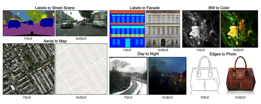
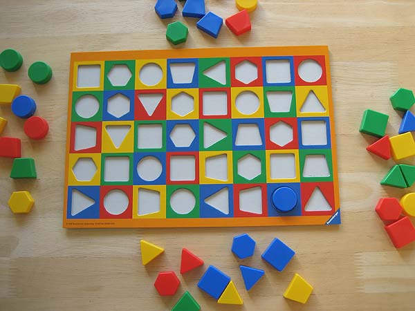
Mapping is a powerful cognitive capability. This collection contains examples of mappings in our everyday life and especially in the manipulation of symbols.
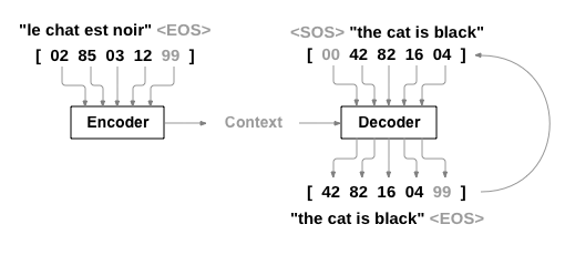
It’s not clearly distinguished between mapping, translation and analogy. Furthermore it’s a wide view on the topic of mapping.

Maps

Names

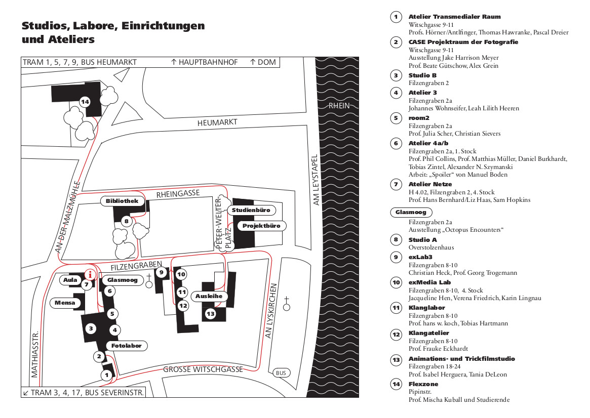
The map above includes names (of persons) as well. Names are another example of mappings. We relate a person to it’s name.

Analogy

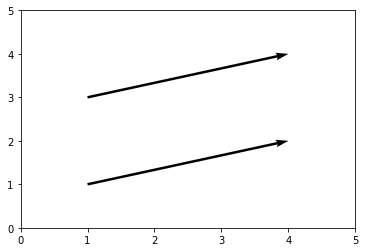
analogy = relation of similarity between two objects, phenomena, beings etc.

analog = comparable by transfer

''' Two analog vectors. '''
import matplotlib.pyplot as plt
xv = 3
yv = 1
plt.quiver([1, 1], [1, 3], [xv, xv], [yv, yv], angles='xy', scale_units='xy', scale=1)
plt.xlim(0, 5)
plt.ylim(0, 5)
plt.show()

Exchange

Accoring to Alfred Sohn-Rethel (In: Das Geld, die bare Münze des Apriori. 1990) the origin of abstract thinking lies in the use of money as a medium for an abstract exchange value. (From [6](4))

Concrete mapping used for trading (like “a sheep for a knive”) is an even older form of mapping and the necessary base for abstract mapping.

Formalization

Money is an example of a formal system. Other examples are language, law, traffic rules. [2](91)

Social media platforms are popular contemporary formal systems.

Algorithms are formal systems.

Formal systems are structures, which are meaningless themselves. Meaning arises when we perform mappings between the formal and the concrete/ when we embed them into the world.

Coordinate system

Geometry is a mapping between the concrete and the formal (and idealized). Concrete properties or actions are the base and are being mapped to abstract terms and ideas. [6](10)

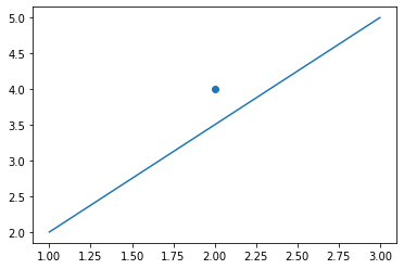
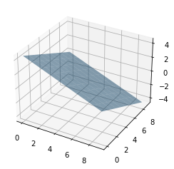
The coordinate system serves as a system to map geometry to computable operations. [6] (12)

import matplotlib.pyplot as plt
import numpy as np

plt.scatter([2], [4]) # dot
plt.plot([1, 3], [2, 5]) # line

# plane
fig = plt.figure()

# add axes
ax = fig.add_subplot(111,projection='3d')

xx, yy = np.meshgrid(range(10), range(10))
z = (9 - xx - yy) / 2 

# plot the plane
ax.plot_surface(xx, yy, z, alpha=0.5)

plt.show()

Instructions

Gregor Weichbrodt: BÆBEL (2015)

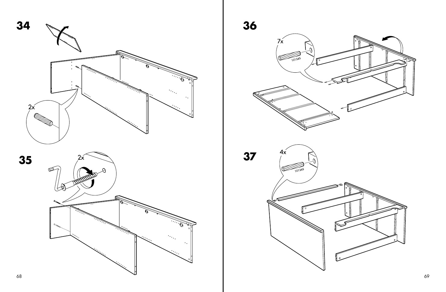
Single pages from IKEA furniture-assembly instructions were mixed together and renumbered. The result is an instructions manual of about 700 pages. (Artist’s website)

“BÆBEL’s name suggests both staggering ambition – and if you followed its instructions, and assembled all IKEA furniture into a single fixture, what could that be but a tower to god? – and its promise of universal comprehension: IKEA’s power is predicated on communicating across languages, which is why its manuals eschew words entirely for these severe and elegant images.” ( Julia Pelta Feldman)

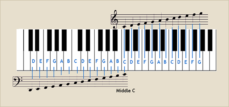
Sheet music

Sounds (and movements to produce them) are mapped to a graphical notation system and backwards.

Mapping between symbols / dictionaries

In the notebook »Programming in Beatnik« we got in touch with ASCII values. Integers are mapped to symbols of the latin alphabet, to arabic numbers 0 to 9 and to some special characters.

# Map character to corresponding ASCII number with ord()
print(ord('a'))

# Map number to corresponding ASCII character with chr()
print(chr(97))

# Nested mapping
print(chr(ord('a')))

97
a
a

When we work with computers we work with many of these mappings/ translations. Other examples are

• the mapping of RGB-values to color

• the translation of images encoded as text into a visible image

• fundamentally the translation (interpretation) of 0 and 1 into numbers and anything above

# Map character > ASCII value > binary value
print(bin(ord('a'))) # '0b' indicates that this string is a binary representation

0b1100001

Vectorization

Neural networks work with numbers, not with characters. If we want to process language, then we have to translate it into numbers - or more specific - into vectors (Vectorization).

Below is an example with an (unfortunately already deprecated) Subword Tokenizer. It doesn’t make much sense because the dataset is way too small.

import tensorflow as tf
import tensorflow_datasets as tfds
import numpy as np
import pandas as pd
import os
import re

# read text
with open(os.getcwd()+'/intro.md', 'r') as f:
    txt = f.read().lower()
    
# remove urls
txt = re.sub('<a[\s\S]*?>', '', txt)
txt = txt.replace('</a>', '')
# remove punctuation and special characters
txt = re.sub(r'[^\w\s]','', txt)
# replace \n
txt = txt.replace('\n', ' ')
# vectorize
txt = txt.split()
txt = [word for word in txt if len(word) > 0]
print(' '.join(txt))

codichte experiments with cognitive systems this book is a documentation of a seminar of the same name given at the academy of media arts cologne in winter 202021 by georg trogemann christian heck and mattis kuhn description through technology we expand our cognitive abilities we try to inscribe our experiences abilities and actions into machine cognitive systems but as soon as we use them they inscribe themselves into our experiences and thus into us in the seminar we experiment with nonhuman cognition and alltoohuman writing techniques with possibility spaces of texts from the library of babel and algorithmic decision making through neural thought vectors and with language hacking machine poetry and poetry machines the seminar focuses on characters words and texts artificial intelligences can do nothing else they are nothing else the material they process are symbols and texts they themselves are also nothing but symbols and texts sense and meaning conclusions and consequences all that follows from the text ie their embedding in the world belongs to the context from this perspective both modernist poetry and modern neuroscience discovered the synaptic space at the beginning of the 20th century the syntax of our formal technical languages artificial neural networks thus entered a new millennium hand in hand with early poetic language techniques and experiments although artificial neural networks are not the focus of our discussion in this seminar we consider them albeit in a larger context as a cognitive system among other cognitive systems since we will go deeper into the syntactic and semantic spaces of these cognitive systems in individual sessions programming skills are helpful but not required to participate in the seminar introductory presentation here you can find a pdf of our introductory presentation

# create dataset
df = pd.DataFrame(txt)
ds = tf.data.Dataset.from_tensor_slices((df))

# create a tokenizer based on the dataset
tokenizer = tfds.deprecated.text.SubwordTextEncoder.build_from_corpus(
    (x.numpy()[0] for x in ds),
    target_vocab_size=400)

# Encode text into integers referring to subwords
encoded_txt = tokenizer.encode(' '.join(txt))
print(encoded_txt)

[26, 49, 50, 20, 171, 116, 171, 9, 171, 8, 171, 21, 171, 30, 171, 132, 250, 246, 171, 44, 171, 236, 171, 125, 238, 60, 121, 27, 102, 171, 3, 171, 236, 171, 11, 171, 3, 171, 1, 171, 254, 134, 240, 171, 94, 22, 171, 113, 16, 249, 171, 27, 171, 1, 171, 56, 236, 25, 248, 260, 171, 3, 171, 22, 49, 236, 171, 28, 255, 254, 171, 26, 97, 38, 171, 4, 171, 58, 34, 24, 171, 138, 138, 189, 188, 171, 237, 260, 171, 46, 250, 253, 242, 171, 61, 250, 46, 41, 249, 249, 171, 50, 80, 72, 244, 55, 171, 45, 238, 246, 171, 2, 171, 96, 255, 44, 171, 246, 256, 243, 249, 171, 25, 78, 80, 83, 13, 171, 63, 171, 68, 250, 97, 260, 171, 6, 171, 118, 2, 171, 7, 171, 8, 171, 137, 171, 6, 171, 61, 260, 171, 10, 171, 104, 171, 7, 171, 117, 171, 137, 171, 2, 171, 136, 101, 171, 23, 171, 40, 171, 8, 171, 21, 171, 51, 171, 53, 171, 76, 13, 171, 53, 171, 6, 171, 17, 240, 171, 66, 171, 18, 171, 104, 171, 65, 171, 23, 171, 7, 171, 117, 171, 2, 171, 62, 171, 23, 171, 17, 171, 4, 171, 1, 171, 11, 171, 6, 171, 118, 120, 22, 34, 171, 9, 171, 249, 13, 110, 171, 26, 242, 249, 43, 102, 171, 2, 171, 135, 10, 250, 110, 171, 258, 79, 105, 171, 67, 171, 9, 171, 86, 73, 237, 107, 43, 260, 171, 74, 171, 3, 171, 19, 171, 47, 171, 1, 171, 98, 237, 81, 253, 260, 171, 3, 171, 237, 236, 133, 171, 2, 171, 5, 112, 79, 243, 39, 238, 171, 25, 238, 44, 102, 171, 41, 99, 171, 63, 171, 37, 171, 64, 255, 171, 16, 238, 10, 253, 254, 171, 2, 171, 9, 171, 42, 171, 243, 56, 99, 171, 40, 171, 33, 171, 2, 171, 33, 171, 40, 254, 171, 1, 171, 11, 171, 114, 119, 171, 13, 171, 50, 28, 136, 24, 254, 171, 57, 239, 254, 171, 2, 171, 19, 171, 54, 171, 4, 20, 14, 244, 46, 93, 254, 171, 131, 171, 125, 171, 35, 171, 123, 171, 18, 171, 15, 171, 35, 171, 123, 171, 1, 171, 96, 120, 5, 171, 18, 171, 84, 130, 254, 254, 171, 15, 171, 70, 171, 2, 171, 19, 171, 18, 171, 65, 171, 15, 171, 5, 76, 171, 35, 171, 51, 171, 70, 171, 2, 171, 19, 171, 12, 249, 12, 171, 2, 171, 22, 55, 105, 171, 26, 249, 238, 247, 17, 101, 171, 2, 171, 129, 240, 82, 122, 254, 171, 135, 171, 31, 27, 171, 115, 14, 250, 258, 254, 171, 47, 171, 1, 171, 20, 259, 255, 171, 108, 171, 1, 100, 171, 48, 52, 239, 49, 36, 171, 4, 171, 1, 171, 57, 247, 239, 171, 133, 89, 254, 171, 10, 171, 1, 171, 128, 171, 47, 171, 30, 171, 87, 75, 240, 127, 16, 171, 132, 31, 171, 95, 44, 255, 171, 33, 171, 2, 171, 95, 171, 38, 59, 250, 78, 108, 93, 171, 126, 250, 16, 32, 239, 171, 1, 171, 71, 94, 83, 238, 171, 75, 56, 240, 171, 27, 171, 1, 171, 52, 113, 91, 36, 171, 3, 171, 1, 171, 138, 31, 171, 130, 34, 59, 260, 171, 1, 171, 69, 259, 171, 3, 171, 7, 171, 115, 253, 41, 247, 171, 68, 244, 238, 5, 171, 42, 254, 171, 54, 171, 37, 171, 92, 171, 62, 171, 121, 24, 124, 171, 236, 171, 38, 258, 171, 39, 14, 240, 91, 60, 171, 111, 171, 4, 171, 111, 171, 9, 171, 240, 28, 247, 260, 171, 86, 240, 29, 171, 42, 171, 67, 171, 2, 171, 116, 171, 5, 64, 171, 54, 171, 37, 171, 92, 171, 15, 171, 90, 171, 1, 171, 114, 171, 3, 171, 7, 171, 126, 17, 77, 171, 4, 171, 30, 171, 11, 171, 6, 171, 129, 109, 24, 171, 66, 171, 5, 52, 43, 171, 4, 171, 236, 171, 247, 28, 46, 253, 171, 128, 171, 53, 171, 236, 171, 8, 171, 71, 72, 48, 171, 134, 89, 171, 250, 1, 253, 171, 8, 171, 21, 171, 254, 4, 130, 171, 6, 171, 58, 14, 171, 112, 171, 25, 240, 87, 171, 23, 171, 1, 171, 69, 127, 238, 171, 2, 171, 12, 41, 34, 244, 238, 171, 74, 171, 3, 171, 1, 12, 171, 8, 171, 21, 171, 4, 171, 106, 244, 257, 109, 256, 5, 171, 12, 73, 13, 254, 171, 84, 242, 81, 248, 39, 36, 171, 254, 246, 107, 247, 254, 171, 15, 171, 45, 247, 251, 241, 256, 247, 171, 51, 171, 90, 171, 32, 82, 100, 124, 171, 10, 171, 88, 253, 29, 244, 88, 20, 171, 4, 171, 1, 171, 11, 171, 103, 171, 85, 171, 45, 32, 171, 260, 250, 256, 171, 131, 171, 241, 106, 171, 236, 171, 251, 239, 241, 171, 3, 171, 7, 171, 103, 171, 85]

# print first tokens as an integer-word-pair
for token in encoded_txt[:74]:
    print('{:3} --> {}'.format(token, tokenizer.decode([token])))

 26 --> co
 49 --> di
 50 --> ch
 20 --> te
171 -->  
116 --> experiments
171 -->  
  9 --> with
171 -->  
  8 --> cognitive
171 -->  
 21 --> systems
171 -->  
 30 --> this
171 -->  
132 --> bo
250 --> o
246 --> k
171 -->  
 44 --> is
171 -->  
236 --> a
171 -->  
125 --> do
238 --> c
 60 --> um
121 --> ent
 27 --> at
102 --> ion
171 -->  
  3 --> of
171 -->  
236 --> a
171 -->  
 11 --> seminar
171 -->  
  3 --> of
171 -->  
  1 --> the
171 -->  
254 --> s
134 --> am
240 --> e
171 -->  
 94 --> na
 22 --> me
171 -->  
113 --> gi
 16 --> ve
249 --> n
171 -->  
 27 --> at
171 -->  
  1 --> the
171 -->  
 56 --> ac
236 --> a
 25 --> de
248 --> m
260 --> y
171 -->  
  3 --> of
171 -->  
 22 --> me
 49 --> di
236 --> a
171 -->  
 28 --> ar
255 --> t
254 --> s
171 -->  
 26 --> co
 97 --> log
 38 --> ne

This subwords’ purpose is to demonstrate the idea behind it. The target_vocab_size=400 is too small. Try 410 (there is some threshold between the numbers) to see the difference. With 410 there are no subwords (just words), meaning that the dataset is too small.

Inventions

The Beatnik programming language uses another mapping system (dictionary). Alphabetical symbols are mapped to numerical values:

SCRABBLE = {
    'A': 1,
    'B': 3,
    'C': 3,
    'D': 2,
    'E': 1,
    'F': 4,
    'G': 2,
    'H': 4,
    'I': 1,
    'J': 8,
    'K': 5,
    'L': 1,
    'M': 3,
    'N': 1,
    'O': 1,
    'P': 3,
    'Q': 10,
    'R': 1,
    'S': 1,
    'T': 1,
    'U': 1,
    'V': 4,
    'W': 4,
    'X': 8,
    'Y': 4,
    'Z': 10
}

This arbitrary values are of course only one possible mapping. Most mappings are inventions. (Which ones are not?) We can easily invent new mappings.

An artistic example:

Benoit Felix: Compter = 17 = Tellen (2014)

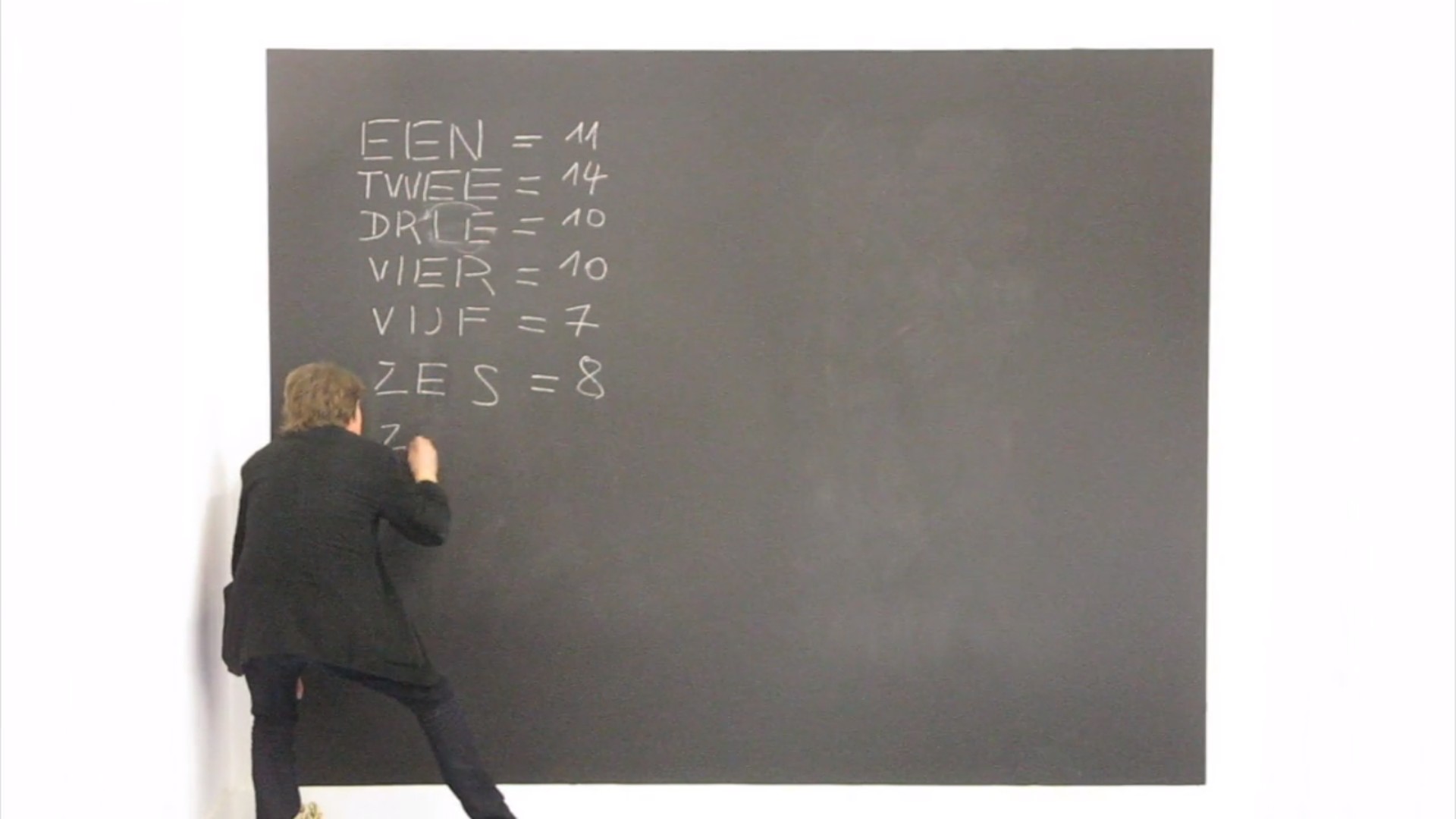
Benoit Felix counts from 1 upwards but writes down the numerals (a mapping) of the numbers. Then he counts the number of strokes necessary to write each numeral and assigns this value to the numeral. But he did it just for French, so there are some possible mappings left.

Beatnik introduces another mapping. Numbers are mapped to actions:

ACTION = {
    5: 'PUSH',
    6: 'DISCARD',
    7: 'ADD',
    8: 'INPUT',
    9: 'OUTPUT',
    10: 'SUBTRACT',
    11: 'SWAP',
    12: 'DUP',
    13: 'SKIP_AHEAD_ZERO',
    14: 'SKIP_AHEAD_NONZERO',
    15: 'SKIP_BACK_ZERO',
    16: 'SKIP_BACK_NONZERO',
    17: 'STOP',
}

Python’s map() function

map() is a built-in function of Python. You can use it to apply a transformation function onto all elements of an iterable (like a list or a dictionary).

In the notebook if-elif-else we wrote a (obsolete) function called swap_case(). It performs a transformation: lower case characters are mapped to their upper case equivalent, vice versa. Now we will see how we can perfrom the same transformation with map().

txt = "»Tender Buttons«, from Gertrude Stein" 

'''
Old function.
'''
def change_case(inp_):
    # create an empty variable
    swapped = ''
    # loop through string
    for character in inp_:
        # if is lower:
        if character.islower():
            # append swapped character
            swapped += character.upper()
        # otherwise it's upper:
        else:
            swapped += character.lower()
    
    # when the loop is finished we return the result
    return swapped

print(change_case(txt))

'''
If we use the map() function we don't need a loop.
The function deals with one value only.
'''
def swap(inp_):
    if inp_.islower():
        return inp_.upper()
    else:
        return inp_.lower()


txt_ = map(swap, txt)
# As map returns an iterable, we have to transform it into a list.
txt_ = list(txt_)
# and then join the items of the list to a string.
txt_ = ''.join(txt_)
print(txt_)

»tENDER bUTTONS«, FROM gERTRUDE sTEIN
»tENDER bUTTONS«, FROM gERTRUDE sTEIN

Mapping in algorithms

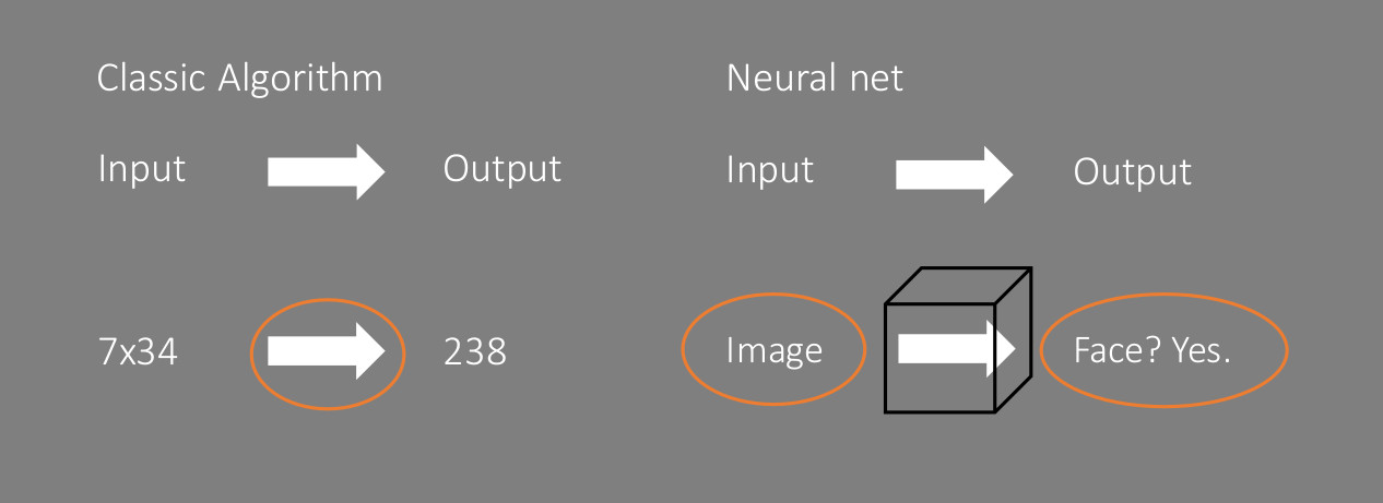
We can think of a classic algorithm in the sense of a mapping. The algorithm maps an input to an output.

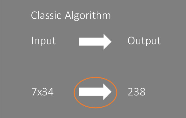
Example: Multiplication

We can imagine different algorithms which perform different actions as long as the mapping is the same.

For example we could do it literally and add 34 7 times (multiply_through_sum).

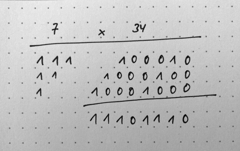
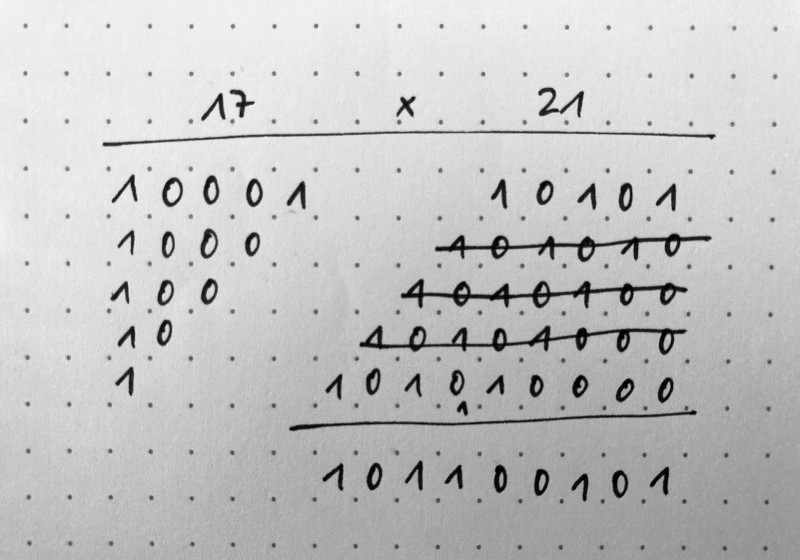
Or we could map our numbers from the decimal numeral system to the binary numeral system and solve the multiplication with a different method (russian_peasant_multiplication).

'''
Add k j times.
'''
def multiply_through_sum(j, k):
    res = 0
    for i in range(j):
        res += k
    return res


'''
Binary Multiplication with Russian Peasant Multiplication
https://en.wikipedia.org/wiki/Multiplication_algorithm#Binary_or_Peasant_multiplication
'''

def russian_peasant_multiplication(a, b):
    
    result = 0
    
    while a > 0:
        rest = a % 2
        if rest == 1:
            result += b
            a -= 1
        b = b << 1
        a = a >> 1
    
    return result
    

print("python's built-in method:", 7*34) 
# Python uses the grade school algorithm (https://en.wikipedia.org/wiki/Multiplication_algorithm#Long_multiplication) for small numbers,
# Karatsuba multiplication for large numbers (https://en.wikipedia.org/wiki/Multiplication_algorithm#Karatsuba_multiplication)
print('multiply through sum:', multiply_through_sum(7, 34))
print('russian peasant multiplication:', russian_peasant_multiplication(7, 34))

python's built-in method: 238
multiply through sum: 238
russian peasant multiplication: 238

Peasant multiplication by hand

print('7 x 34 =', 7*34)
print('11101110 =', int('11101110', 2))

print('17 x 21 =', 17*21)
print('101100101 =', int('101100101', 2))

7 x 34 = 238
11101110 = 238
17 x 21 = 357
101100101 = 357

Example: Sorting

Sorting is a more obvious example for mapping. We map a sequence like [0, 5, 3, 2, 2] to a sequence like [0, 2, 2, 3, 5].

Different algorithms perform this task in different ways, but the mapping (relation) has to be always the same.

'''
Insertion sort.
https://github.com/TheAlgorithms/Python/blob/master/sorts/insertion_sort.py
'''

def insertion_sort(collection: list) -> list:
    """A pure Python implementation of the insertion sort algorithm
    :param collection: some mutable ordered collection with heterogeneous
    comparable items inside
    :return: the same collection ordered by ascending
    Examples:
    >>> insertion_sort([0, 5, 3, 2, 2])
    [0, 2, 2, 3, 5]
    >>> insertion_sort([])
    []
    >>> insertion_sort([-2, -5, -45])
    [-45, -5, -2]
    """

    for loop_index in range(1, len(collection)):
        insertion_index = loop_index
        while (
            insertion_index > 0
            and collection[insertion_index - 1] > collection[insertion_index]
        ):
            collection[insertion_index], collection[insertion_index - 1] = (
                collection[insertion_index - 1],
                collection[insertion_index],
            )
            insertion_index -= 1
# changed: print progress 
            print(collection)

    return collection


'''
Quick sort.
https://github.com/TheAlgorithms/Python/blob/master/sorts/quick_sort.py
'''

def quick_sort(collection):
    """Pure implementation of quick sort algorithm in Python
    :param collection: some mutable ordered collection with heterogeneous
    comparable items inside
    :return: the same collection ordered by ascending
    Examples:
    >>> quick_sort([0, 5, 3, 2, 2])
    [0, 2, 2, 3, 5]
    >>> quick_sort([])
    []
    >>> quick_sort([-2, -5, -45])
    [-45, -5, -2]
    """
    length = len(collection)
    if length <= 1:
        return collection
    else:
        # Use the last element as the first pivot
        pivot = collection.pop()
        # Put elements greater than pivot in greater list
        # Put elements lesser than pivot in lesser list
        greater, lesser = [], []
        for element in collection:
            if element > pivot:
                greater.append(element)
            else:
                lesser.append(element)
# changed: print progress                
            print(lesser, pivot, greater)
        return quick_sort(lesser) + [pivot] + quick_sort(greater)
    
    
import random
sequence = [x for x in range(10)]
random.shuffle(sequence)
print('unordered sequence:', sequence, '\n')
print('insertion sort progress:\n')
print('\nsorted sequence:', insertion_sort(sequence), '\n')
print('quick sort progress:\n')
print('\nsorted sequence:', quick_sort(sequence))

unordered sequence: [0, 4, 3, 6, 5, 8, 1, 7, 9, 2] 

insertion sort progress:

[0, 3, 4, 6, 5, 8, 1, 7, 9, 2]
[0, 3, 4, 5, 6, 8, 1, 7, 9, 2]
[0, 3, 4, 5, 6, 1, 8, 7, 9, 2]
[0, 3, 4, 5, 1, 6, 8, 7, 9, 2]
[0, 3, 4, 1, 5, 6, 8, 7, 9, 2]
[0, 3, 1, 4, 5, 6, 8, 7, 9, 2]
[0, 1, 3, 4, 5, 6, 8, 7, 9, 2]
[0, 1, 3, 4, 5, 6, 7, 8, 9, 2]
[0, 1, 3, 4, 5, 6, 7, 8, 2, 9]
[0, 1, 3, 4, 5, 6, 7, 2, 8, 9]
[0, 1, 3, 4, 5, 6, 2, 7, 8, 9]
[0, 1, 3, 4, 5, 2, 6, 7, 8, 9]
[0, 1, 3, 4, 2, 5, 6, 7, 8, 9]
[0, 1, 3, 2, 4, 5, 6, 7, 8, 9]
[0, 1, 2, 3, 4, 5, 6, 7, 8, 9]

sorted sequence: [0, 1, 2, 3, 4, 5, 6, 7, 8, 9] 

quick sort progress:

[0] 9 []
[0, 1] 9 []
[0, 1, 2] 9 []
[0, 1, 2, 3] 9 []
[0, 1, 2, 3, 4] 9 []
[0, 1, 2, 3, 4, 5] 9 []
[0, 1, 2, 3, 4, 5, 6] 9 []
[0, 1, 2, 3, 4, 5, 6, 7] 9 []
[0, 1, 2, 3, 4, 5, 6, 7, 8] 9 []
[0] 8 []
[0, 1] 8 []
[0, 1, 2] 8 []
[0, 1, 2, 3] 8 []
[0, 1, 2, 3, 4] 8 []
[0, 1, 2, 3, 4, 5] 8 []
[0, 1, 2, 3, 4, 5, 6] 8 []
[0, 1, 2, 3, 4, 5, 6, 7] 8 []
[0] 7 []
[0, 1] 7 []
[0, 1, 2] 7 []
[0, 1, 2, 3] 7 []
[0, 1, 2, 3, 4] 7 []
[0, 1, 2, 3, 4, 5] 7 []
[0, 1, 2, 3, 4, 5, 6] 7 []
[0] 6 []
[0, 1] 6 []
[0, 1, 2] 6 []
[0, 1, 2, 3] 6 []
[0, 1, 2, 3, 4] 6 []
[0, 1, 2, 3, 4, 5] 6 []
[0] 5 []
[0, 1] 5 []
[0, 1, 2] 5 []
[0, 1, 2, 3] 5 []
[0, 1, 2, 3, 4] 5 []
[0] 4 []
[0, 1] 4 []
[0, 1, 2] 4 []
[0, 1, 2, 3] 4 []
[0] 3 []
[0, 1] 3 []
[0, 1, 2] 3 []
[0] 2 []
[0, 1] 2 []
[0] 1 []

sorted sequence: [0, 1, 2, 3, 4, 5, 6, 7, 8, 9]

Sortieren ist nahe am Vergleichen. Vergleich wird genutzt zum Sortieren.

For a mapping of sort algorithms to sounds see: Shintaro Miyazaki: Sorting Algorithms

Sorting is also used as a strategy in artistic projects. One example:

Timo Klos: ON THE SURFACE

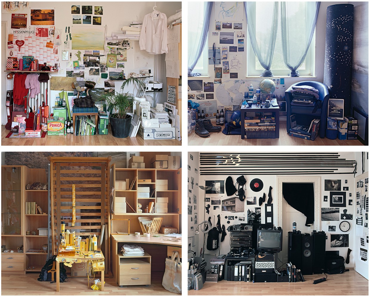
“I matched my room up to colours. It looks beautiful, tidy and I find the things I am searching for. However, there are many processes which doesn’t work anymore. For example it is impossible to listen to Music, because the audio cables lie in the yellow brownish corner whereas the amplifier belongs to the black part of the room.” (Artist’s website)

Another aspect of the image below is the directional arrow. Most algorithms are “Einbahnstraßen” (one-way roads). [4] (103)

We can’t apply the sort algorithms to reestablish the original order.

Beatnik instead maps symbols in a bidirectional way. At least in our mind as sophisticated beatnik programmers. We think forwards from our code to the output it produces (through values and actions) and backwards from our planned output to the necessary code.

Mapping in CGI

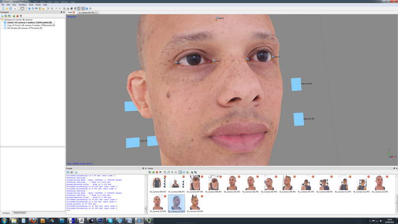
A texture is mapped on an object.

(source)

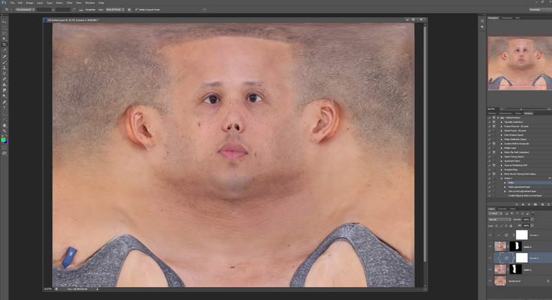
Martina Menegon: It suits me well (2016)

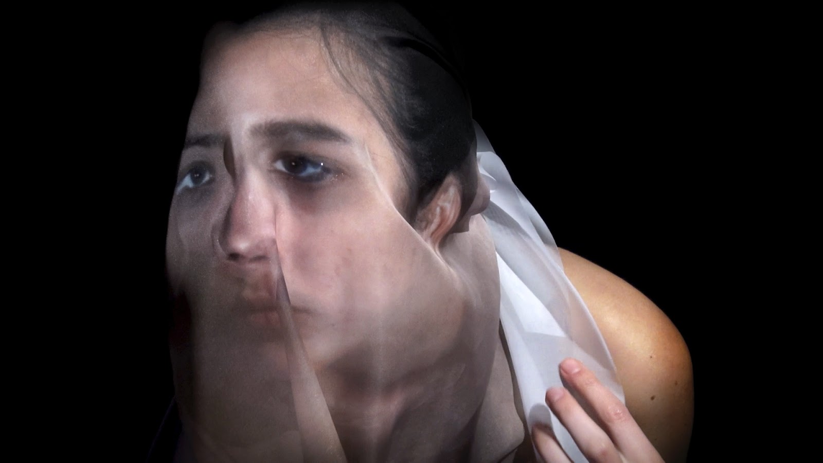
The UV map texture of the artist’s scanned body is printed on a semi-transparent soft cloth. In a room, alone, the artist recorded herself wearing the cloth, attempting to overlap the right scanned part of her printed body with her real one. “It Suits Me Well” is a video loop, in which the body is re-materialised, transformed into a fluid one that oscillates between virtual and physical realities. (Artist’s website)

Mapping genotype to phenotype

Heather Dewey-Hagborg: Stranger Visions (2016)

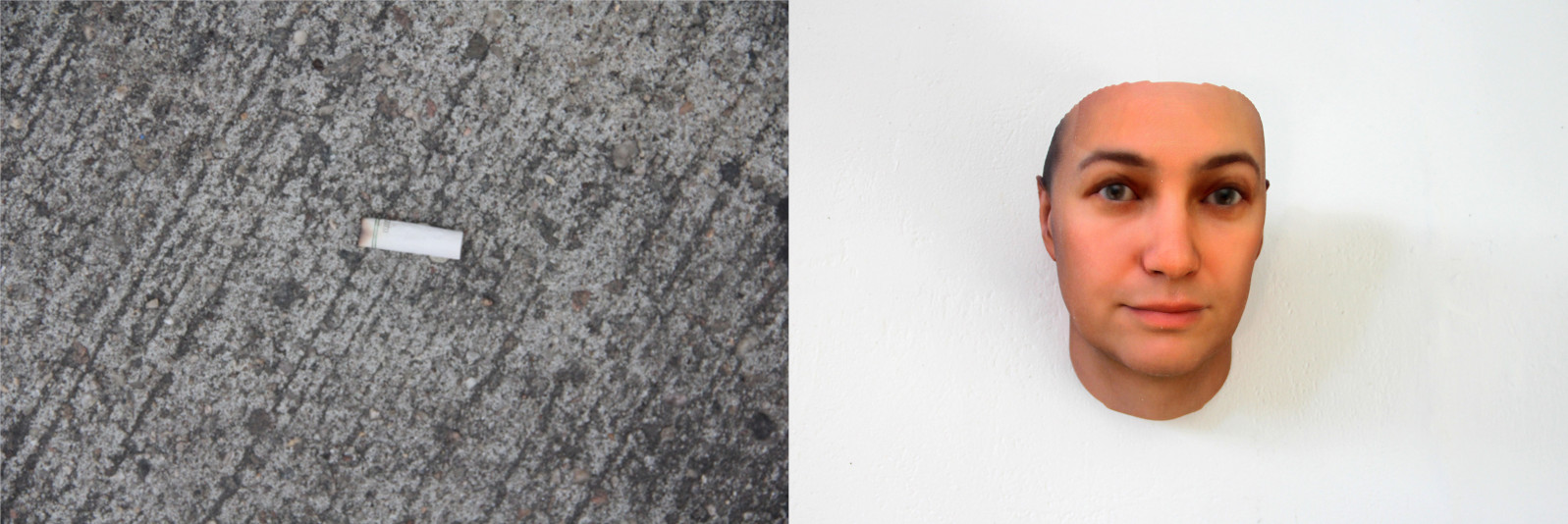
In Stranger Visions I collected hairs, chewed up gum, and cigarette butts from the streets, public bathrooms and waiting rooms of New York City. I extracted DNA from them and analyzed it to computationally generate 3d printed life size full color portraits representing what those individuals might look like, based on genomic research. Working with the traces strangers unwittingly left behind, the project was meant to call attention to the developing technology of forensic DNA phenotyping, the potential for a culture of biological surveillance, and the impulse towards genetic determinism. (Artist’s website)

Mapping in ML

The strength of current machine learning “is to learn and reproduce mappings between inputs and outputs”. [5](49)

In the previous code examples we have written the code. So we have defined the process that establishes the mapping between input and output. We have defined this relation.

Mapping becomes more obvious when we look at some current machine learning algorithms. In the training process we define the mapping through the input and the corresponding output. The neural net computes a relation to map them.

Classification

Classification is not only done through mapping, classification is a mapping itself.
Classification is a very useful cognitive capability to orient oneself in the world.

(Source)

Shinseungback Kimyonghun: Animal Classifier (2016)

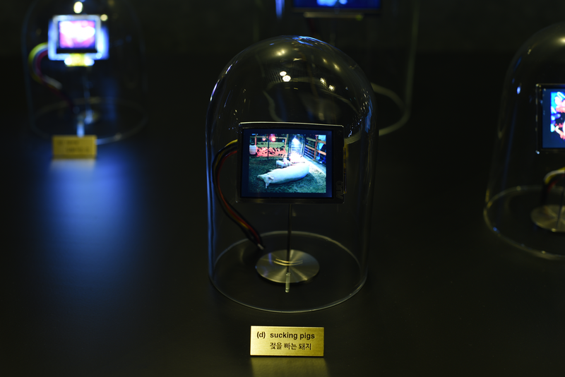
‘Animal Classifier’ is an AI trained to divide animals into the following 14 categories: (a) belonging to the emperor, (b) embalmed, (c) tame, (d) sucking pigs, (e) sirens, (f) fabulous, (g) stray dogs, (h) included in the present classification, (i) frenzied, (j) innumerable, (k) drawn with a very fine camel hair brush, (l) et cetera, (m) having just broken the water pitcher, (n) that from a long way off look like flies.

The taxonomy is from the essay ‘The Analytical Language of John Wilkins’ by Jorge Luis Borges where he writes “it is clear that there is no classification of the Universe not being arbitrary and full of conjectures. The reason for this is very simple: we do not know what thing the universe is.” He introduces the classification as an example of faulty human schemes. (Artist’s website)

Generative Adversarial Network (GAN)

(Source)

More examples of mapping in ML

Style Transfer

(Source)

Pix2Pix

(Source)

Seq2Seq

(Source)

Analogies

Word Embedding makes use of analogies between vectors.

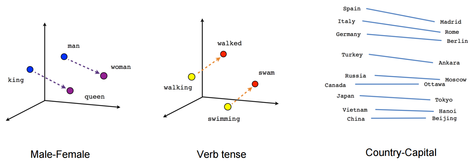(Source) (Further Reading) (Further Reading)

But keep in mind that this visualization itself is a mapping. Embedding vectors have higher dimensions (approximately between 128 and 300). The image shows a mapping into a 3-dimensional space.

Relations

Previously we used the definition of analogy as:

relation of similarity between two objects, phenomena, beings etc.

The following two drawings may be used to see some relations.

• concept: one artist made a drawing on one page and the other one has to respond to this page with an own (related) drawing

• we as viewers can imagine how the lines of the drawings continue and connect to each other

• furthermore it shows a mapping between human and machine actions

• the drawings ask for an interpretation of the relation between the two pages and between us and the drawing

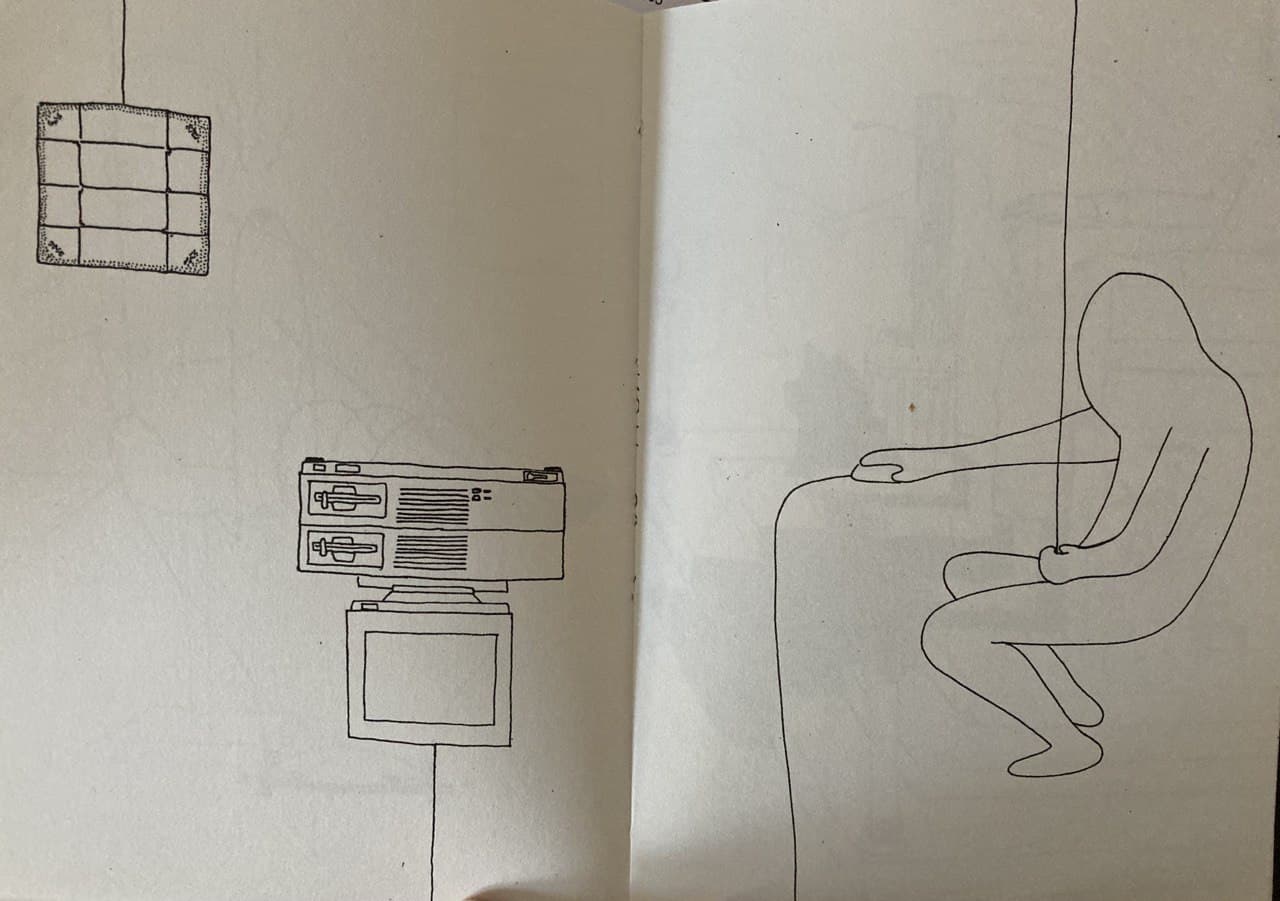
Felix Reutzel & Felix Hofmann-Wissner: Geteilte Freud (2016)

Human-Machine-Interface

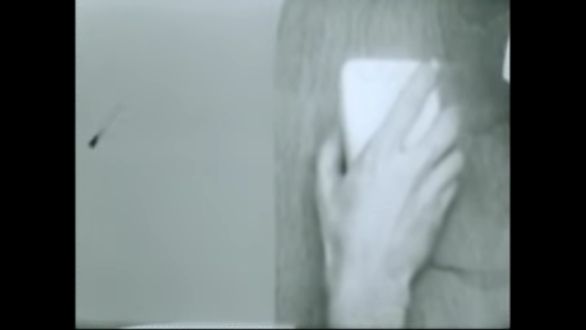
Douglas Engelbart demonstrating the first Computer Mouse. We see a mapping of physical movements to numbers to virtual movements on a screen.

In Engelbart’s view our intelligence relies on our tools and methods, which are artificial.

“In a very real sense, the development of »artificial intelligence« has been going on for centuries.” (Engelbart, Douglas C. „Augmenting Human Intellect: A Conceptual Framework“.)

Mapping as a cognitive extension

In this manner we can look at mappings as a form of cognitive extensions which enable us to do things easier, faster or at all. For e.g. we can look at multiplication methods as a form of cognitive extension.

In multiplication as learned in school we map numbers to a spatial order and process them in relation to their position.

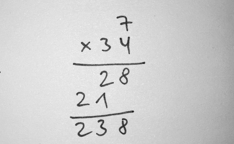
This is just one obvious example but in fact most of the mappings given in this document are cognitive extensions.

Mapping in artistic practice

Especially in media art where we already deal with the digital, mappings are used frequently, mainly to map one quantity to another.

Tega Brain: Being Radiotropic (2016)

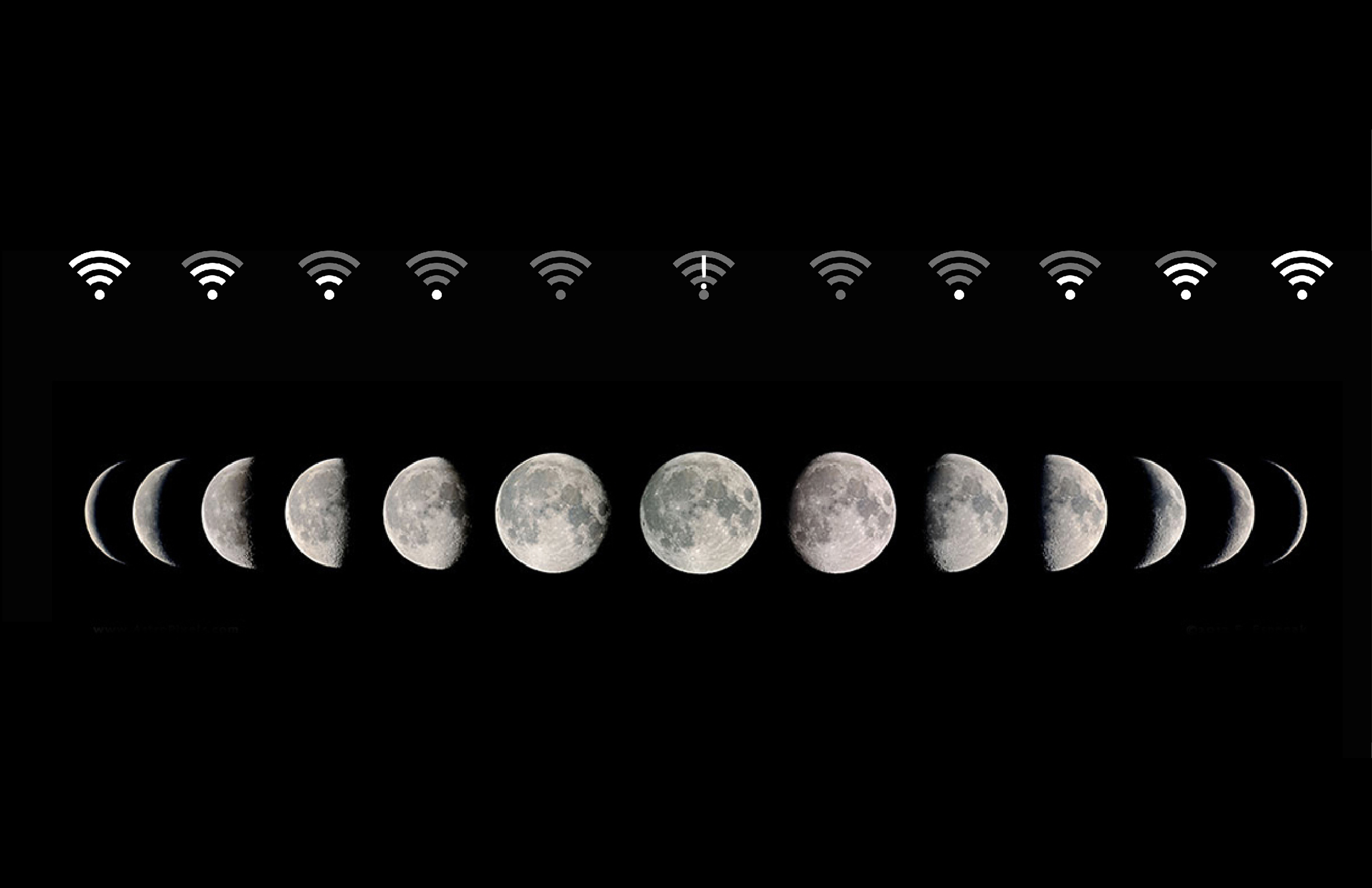
The image shows one part of the work: An Orbit.

An Orbit is a router that couples signal strength with moon phase. For one day per month it provides maximum wifi signal, and for one day a month it provides no network at all. Between these points the signal waxes and wanes, oscillating over a 28 day period. (Artist’s website)

Traduktionismus

As mentioned above Mapping is a common strategy in artistic practice. Christian Janecke describes this with the term Traduktionismus (understood as translation). While the aim of a common translation is to remain accurate to the original, it seems that the artistic aim is to create translations “as curious or devious as possible” (translated by the author). [3]

Meaning: if you use mapping in artistic practice, make it good.

Mapping to produce meaning

“Words do not have meaning, they are cues to meaning.” (Elman, J. 2004. An alternative view of the mental lexicon. Quoted from Clark, A. 2008. Supersizing the Mind. 54)

Symbols themselves are meaningless. We connect them with meaning through mapping. This mapping is not written into the symbols. It’s outside of them. Different mappings can result in different meanings. [1](148)

“all meaning is mapping-mediated, which is to say, all meaning comes from analogies.” [1](158) (See also: Hofstadter & Sander: Surfaces and Essences : Analogy as the Fuel and Fire of Thinking (2013).)

Artworks provoking reconfigurations of mappings

If meaning arises from mapping and the interpretation of an aesthetic artifact is the ongoing search for possible (often ambivalent) meanings,
we could look at artworks as a form of challenging existing mappings (or on a higher level: the construction of meaning itself).

Johannes Kreidler: Sheet Music

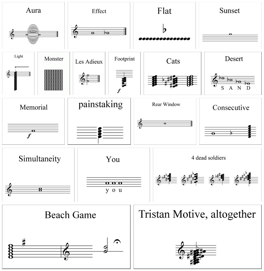
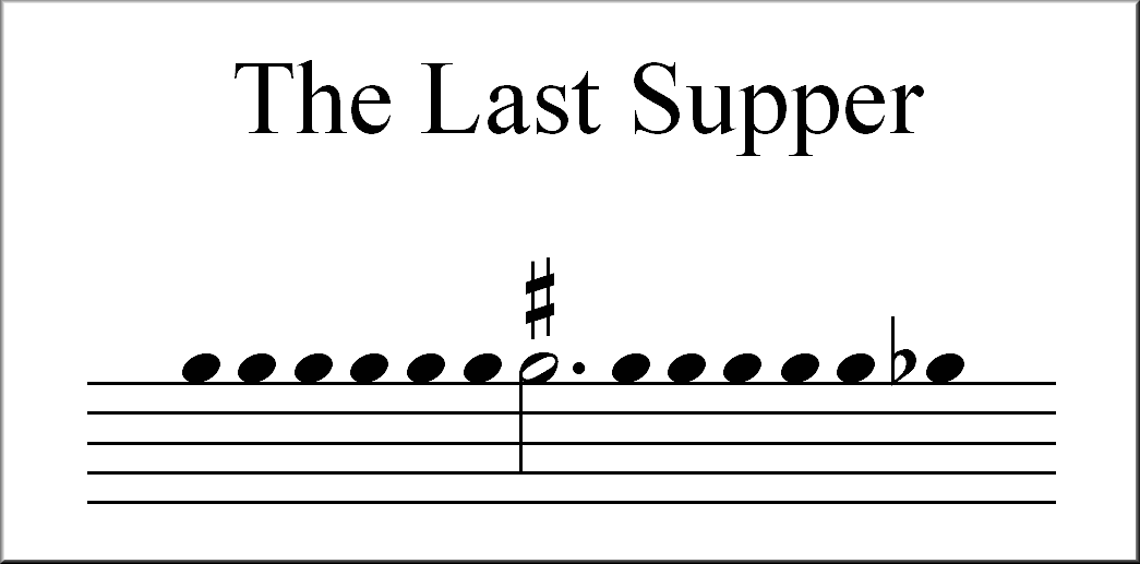
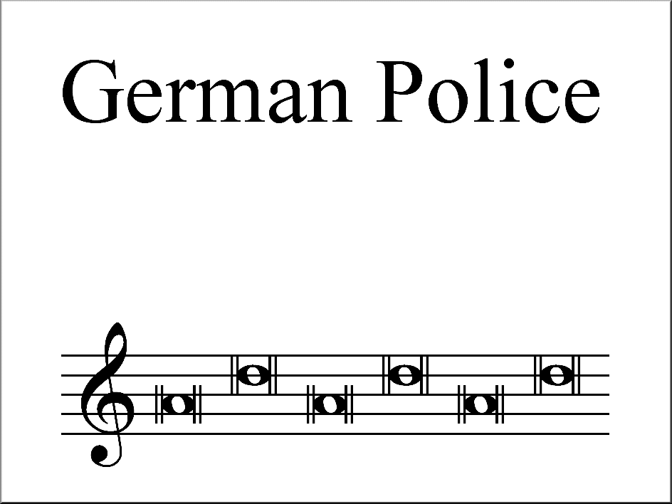
(You can almost hear the siren (or a mapping of that sound) through mapping this notes and the title to memories of the sound, stored in your body.)

Koen Theys: Big String (2004)

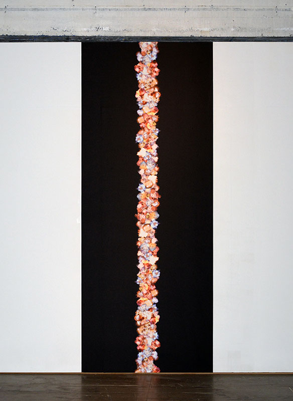
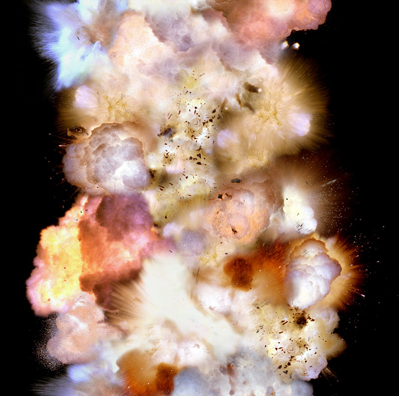
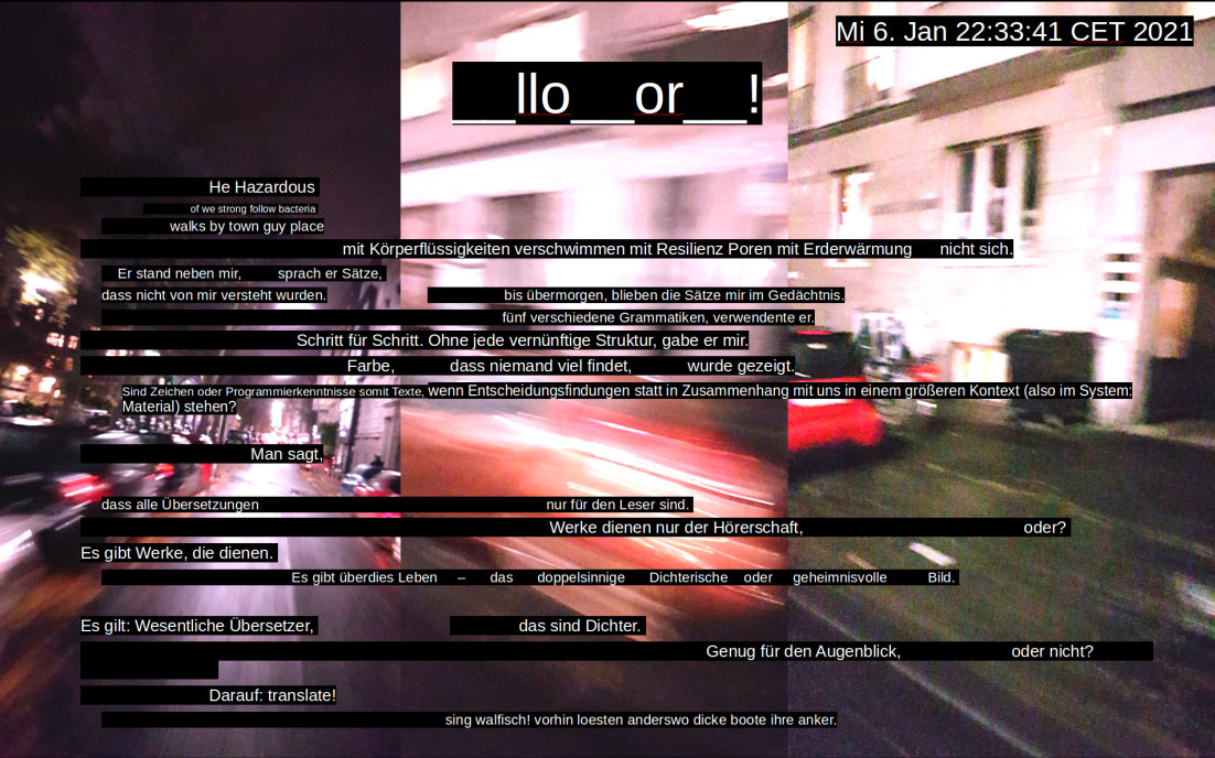
Maybe this questioning of existing mappings becomes even more obvious when we think about poetry.

References

1(1,2)

Douglas R. Hofstadter. I Am a Strange Loop. Basic Books, New York, 2007.

2

Eggert Holling and Peter Kempin. Identität, Geist und Maschine. Rowohlt Taschenbuch Verlag, Reinbek bei Hamburg, 1989.

3

Christian Janecke. Maschen der Kunst. zu Klampen Verlag, Springe, 2011.

4

Shintaro Miyazaki. Algorhythmisiert. Eine Medienarchäologie digitaler Signale und (un)erhörter Zeiteffekte. Kulturverlag Kadmos, Berlin, 2013.

5

Brian Cantwell Smith. The Promise of Artificial Intelligence. Reckoning and Judgment. MIT Press, Cambridge, Massachusetts, 2019.

6(1,2,3)

Georg Trogemann. Die Fülle des Konkreten am Skelett des Formalen. über Abstraktion und Konkretisierung im algorithmischen Denken und Tun. 2014. URL: http://georgtrogemann.de/wp-content/uploads/2016/02/Trogemann_Fu%CC%88lleDesKonkreten-2014.pdf.

Adversarial Hacking Introduction to Programming with Python